A Basic Approach to the Expectation-Maximization Algorithm

Two Biased Coins

Author: Ali Nawaf


Date: September 5, 2025

---

Introduction

The Expectation-Maximization (EM) algorithm is an iterative method for finding maximum likelihood estimates of parameters in statistical models that depend on unobserved, or latent, variables. It alternates between performing an expectation (E) step, which creates a function for the expectation of the log-likelihood evaluated using the current estimate for the parameters, and a maximization (M) step, which computes parameters maximizing the expected log-likelihood found in the E-step. These new parameters are then used in the subsequent E-step.

In machine learning, the EM algorithm is a fundamental tool for unsupervised learning. It is the core mechanism behind clustering algorithms like Gaussian Mixture Models (GMMs) and is used in various fields, from natural language processing to computer vision, for problems involving missing data.

---

Problem Definition

We consider a simple experiment involving two biased coins, Coin A and Coin B. The true, hidden probability of each coin landing on Heads is:

• Coin A: $\pi_A = 0.80$
• Coin B: $\pi_B = 0.30$

For any given flip, both coins are equally likely to be chosen, meaning the probability of selecting either coin is $P(\text{Choose A}) = P(\text{Choose B}) = 0.5$. Our goal is to estimate the hidden biases $\pi_A$ and $\pi_B$ using only a sequence of observed outcomes (Heads or Tails), without knowing which coin was used for which flip.

---

Mathematical Formulation

The algorithm iterates between an E-step and an M-step to converge on the most likely parameters. Let our observed data be $X = \{x_1, x_2, \dots, x_N\}$, where $x_i=1$ for Heads and $x_i=0$ for Tails.

E-Step: Calculating Responsibilities

In the E-step, we calculate the posterior probability, or "responsibility," that each coin has for each observation, given our current parameter estimates $\theta = (\pi_A, \pi_B)$.

The responsibility of Coin A for observation $x_i$, denoted $\gamma(z_i = A)$, is calculated as:

$$\gamma(z_i = A) = P(\text{Coin A} \mid x_i, \theta) = \frac{P(x_i \mid \text{A}, \theta) \, P(\text{A})} {P(x_i \mid \text{A}, \theta) \, P(\text{A}) + P(x_i \mid \text{B}, \theta) \, P(\text{B})}.$$

Given our assumption that $P(A) = P(B) = 0.5$, this simplifies to:

$$\gamma(z_i = A) = \frac{P(x_i \mid \pi_A)}{P(x_i \mid \pi_A) + P(x_i \mid \pi_B)}.$$

Where:

• $P(x_i=1 \mid \pi_A) = \pi_A$
• $P(x_i=0 \mid \pi_A) = 1 - \pi_A$.

The responsibility for Coin B is simply:

$$\gamma(z_i = B) = 1 - \gamma(z_i = A).$$

---

M-Step: Maximizing the Likelihood

In the M-step, we use the responsibilities to calculate new, improved estimates for our parameters.

For Coin A, the update is:

$$\pi_A^{\text{new}} = \frac{\sum_{i=1}^{N} \gamma(z_i=A) \cdot x_i}{\sum_{i=1}^{N} \gamma(z_i=A)}.$$

For Coin B, the update is:

$$\pi_B^{\text{new}} = \frac{\sum_{i=1}^{N} \big(1-\gamma(z_i=A)\big) \cdot x_i}{\sum_{i=1}^{N} \big(1-\gamma(z_i=A)\big)}.$$

---

Example: First Iteration

Let's assume an initial guess of $\pi_A^{(0)} = 0.6$ and $\pi_B^{(0)} = 0.4$.

• For an observation of Heads ($x_i=1$):

$$\gamma(z_i=A) = \frac{0.6}{0.6 + 0.4} = 0.6.$$

• For an observation of Tails ($x_i=0$):

$$\gamma(z_i=A) = \frac{1 - 0.6}{(1 - 0.6) + (1 - 0.4)} = \frac{0.4}{0.4 + 0.6} = 0.4.$$

If our 100-flip dataset has 58 Heads and 42 Tails, the soft counts are:

• Total Heads A = $58 \times 0.6 = 34.8$
• Total Tails A = $42 \times 0.4 = 16.8$
• Total Heads B = $58 \times (1-0.6) = 23.2$
• Total Tails B = $42 \times (1-0.4) = 25.2$

The new parameter estimates after one iteration are:

$$\pi_A^{(1)} = \frac{34.8}{34.8 + 16.8} = \frac{34.8}{51.6} \approx 0.674,$$ $$\pi_B^{(1)} = \frac{23.2}{23.2 + 25.2} = \frac{23.2}{48.4} \approx 0.479.$$

---

Final Output

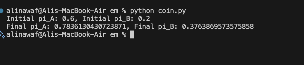
After running the algorithm for 100 iterations with a good initial guess (e.g., $\pi_A=0.8, \pi_B=0.2$) on the provided 100-flip dataset, the parameters converge to values that are very close to the actual probabilities present in the random sample.

The final estimated parameters were:

• Final $\pi_A$: $\approx 0.868$
• Final $\pi_B$: $\approx 0.292$

---

Limitations of this Method

The most significant limitation of the EM algorithm is its sensitivity to initial values. The algorithm is a "hill-climbing" method that seeks to find the peak of the log-likelihood landscape. If this landscape has multiple peaks (a global maximum and several local maxima), the algorithm is only guaranteed to find the top of the peak it starts nearest to.

A poor initial guess can cause the algorithm to converge to a suboptimal local maximum, yielding incorrect parameter estimates. This is illustrated in the figure below, where a good initial guess finds the correct solution, while a bad guess gets stuck in a poor, local maximum.

To mitigate this, the standard practice is to run the algorithm multiple times with different random starting points and choose the result that yields the highest final log-likelihood.

| Good Run |

| Bad Run |

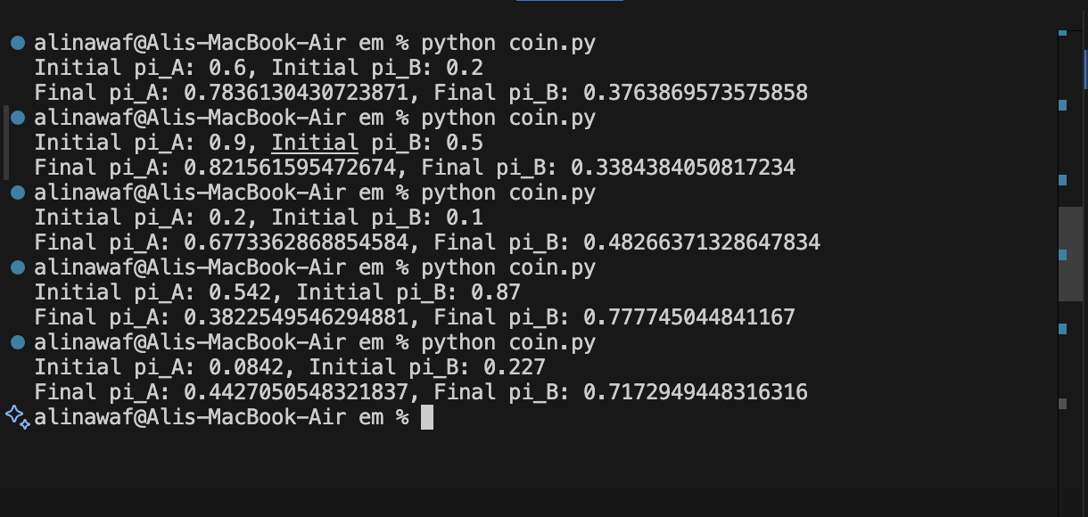
| Figure 1: Convergence plots for two runs. First one : A good initial guess (e.g., 0.8, 0.2) finds the global maximum. The Second: A bad initial guess (e.g., 0.2, 0.1) gets stuck in a suboptimal local maximum. |