Uncovering Hidden Clusters: A Hands-On Guide to the EM Algorithm for Gaussian Mixture Models

Author: Ali Nawaf
Date: September 6, 2025

---

Abstract

This paper documents the implementation of the Expectation-Maximization (EM) algorithm to fit a Gaussian Mixture Model (GMM) to synthetic data. We explore the algorithm's theoretical foundation, from the probabilistic definition of a GMM to the iterative E-step and M-step. Through a practical implementation in Python, we demonstrate how the algorithm can uncover hidden cluster structures. We also confront a key challenge of the EM algorithm: its sensitivity to initialization and the problem of converging to suboptimal local maxima, illustrating how different random starts can lead to dramatically different results.

---

My Implementation Journey

Unsupervised clustering is a fundamental problem in machine learning: how can we find meaningful groups in data without any pre-existing labels? A powerful answer to this is the Gaussian Mixture Model (GMM), which assumes that the data is generated from a mix of several Gaussian (or normal) distributions. The challenge, however, is to find the parameters of these hidden distributions.

This is where the Expectation-Maximization (EM) algorithm comes in. It provides an elegant iterative approach to solve this problem. For this project, I implemented the GMM-EM algorithm from scratch using Python.

My process began by creating a synthetic dataset using scikit-learn's make_blobs function, which gave me a clear ground truth to evaluate my final results. The core of the implementation was the run_em_step function, which contains the two-step dance of the algorithm:

1. The E-Step (Expectation): Calculate the "responsibility" each Gaussian component takes for each data point. This is a soft, probabilistic assignment.
2. The M-Step (Maximization): Use these soft assignments to update the parameters of each Gaussian (its size, center, and shape) to better fit the data it's responsible for.

By repeating these two steps, the model iteratively refines its parameters, converging on a solution that maximizes the likelihood of the observed data.

---

The Mathematical Heart of GMM-EM

To understand the implementation, we must first define the mathematics. A GMM models the probability of a data point x as a weighted sum of $K$ Gaussian components.

Multivariate Gaussian PDF

Each component is a multivariate Gaussian distribution, $\mathcal{N}(\mathbf{x} | \boldsymbol{\mu}_k, \boldsymbol{\Sigma}_k)$, with its own mean $\boldsymbol{\mu}_k$ and covariance matrix $\boldsymbol{\Sigma}_k$. Its probability density function is:

$$\mathcal{N}(\mathbf{x} | \boldsymbol{\mu}_k, \boldsymbol{\Sigma}_k) = \frac{1}{\sqrt{(2\pi)^d |\boldsymbol{\Sigma}_k|}} \exp\left(-\frac{1}{2}(\mathbf{x}-\boldsymbol{\mu}_k)^T \boldsymbol{\Sigma}_k^{-1} (\mathbf{x}-\boldsymbol{\mu}_k)\right)$$

where $d$ is the dimension of the data.

The E-Step: Responsibility

The responsibility of cluster $k$ for data point $\mathbf{x}_i$, denoted $\gamma_{ik}$, is the posterior probability $P(z_i=k | \mathbf{x}_i)$. It is calculated using Bayes' theorem:

$$\gamma_{ik} = \frac{\pi_k \mathcal{N}(\mathbf{x}_i | \boldsymbol{\mu}_k, \boldsymbol{\Sigma}_k)}{\sum_{j=1}^{K} \pi_j \mathcal{N}(\mathbf{x}_i | \boldsymbol{\mu}_j, \boldsymbol{\Sigma}_j)}$$

where $\pi_k$ is the mixing coefficient, or the prior probability of choosing cluster $k$.

The M-Step: Parameter Updates

Using the responsibilities $\gamma_{ik}$ from the E-step, we update the parameters. Let $N_k = \sum_{i=1}^{N} \gamma_{ik}$ be the "soft count" of points in cluster $k$.

$$\boldsymbol{\mu}_k^{\text{new}} = \frac{1}{N_k} \sum_{i=1}^{N} \gamma_{ik} \mathbf{x}_i$$ $$\boldsymbol{\Sigma}_k^{\text{new}} = \frac{1}{N_k} \sum_{i=1}^{N} \gamma_{ik} (\mathbf{x}_i - \boldsymbol{\mu}_k^{\text{new}})(\mathbf{x}_i - \boldsymbol{\mu}_k^{\text{new}})^T$$ $$\pi_k^{\text{new}} = \frac{N_k}{N}$$

where $N$ is the total number of data points.

The Log-Likelihood

The objective is to maximize the log-likelihood of the observed data, which is given by:

$$\ln P(X | \pi, \mu, \Sigma) = \sum_{i=1}^{N} \ln \left( \sum_{k=1}^{K} \pi_k \mathcal{N}(\mathbf{x}_i | \boldsymbol{\mu}_k, \boldsymbol{\Sigma}_k) \right)$$

The EM algorithm is guaranteed to increase this value at every iteration.

---

The Challenge of the Lucky Start: Local Maxima

The EM algorithm is a hill-climbing method. It tries to find the highest peak on a complex "likelihood landscape." However, if this landscape has multiple peaks (a global maximum and several smaller, local maxima), the algorithm's success depends entirely on where it starts. An unlucky random initialization can cause it to climb the wrong hill and get stuck in a suboptimal solution.

This is precisely what happened in one of my experimental runs. With a random seed of 49, the algorithm converged to a solution where two of the true clusters were merged into one.

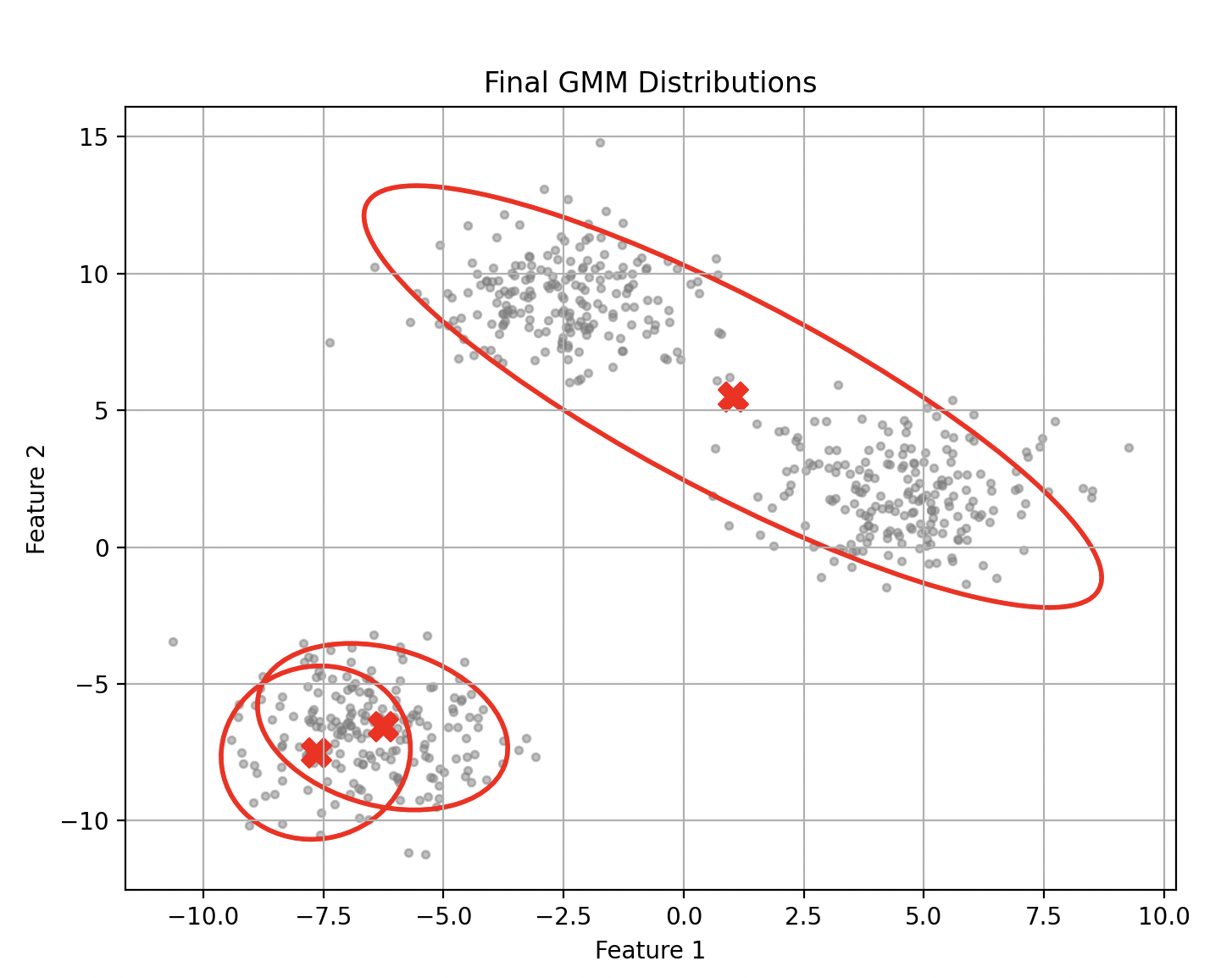An "unlucky" run (ARI = 0.56) where two clusters are incorrectly merged due to a poor initialization.

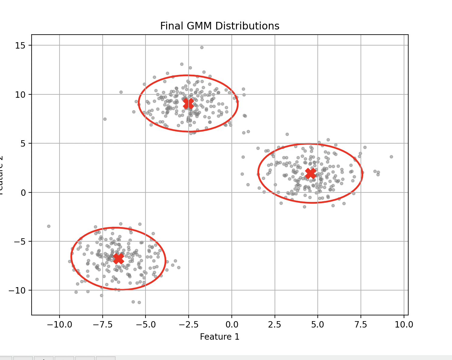
A "lucky" run (ARI = 1.0) where the algorithm correctly identifies all three clusters.

The convergence plot for the unlucky run shows that the algorithm did converge and maximize its likelihood, but it found the peak of the wrong hill. This highlights the critical need to not rely on a single run. The standard mitigation strategy is to perform multiple random starts and select the model that results in the highest final log-likelihood.

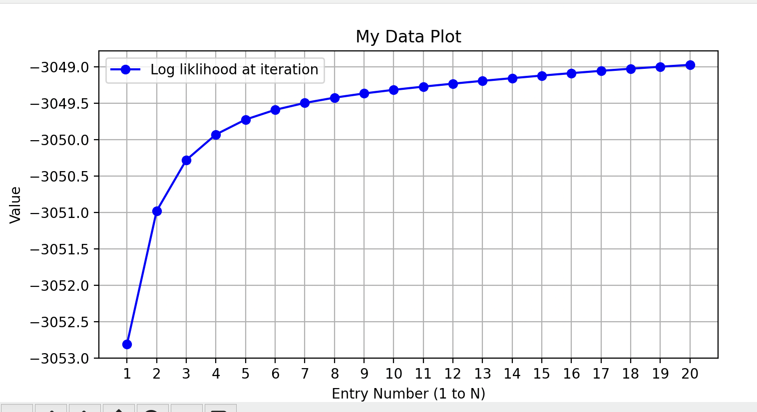
The log-likelihood plot for the unlucky run. The algorithm correctly increases the log-likelihood at each step and converges, but the final solution is a suboptimal local maximum.

---

Conclusion

Implementing the EM algorithm for Gaussian Mixture Models from scratch is a rewarding exercise that provides deep insight into unsupervised learning. The process demonstrates the power of this iterative method to uncover hidden structure in data. However, it also reveals its primary weakness: a sensitivity to initialization that can lead to convergence in local maxima. This underscores the importance of robust implementation strategies, such as multiple random starts, to ensure that the discovered solution is not just a good one, but the best one.