Variational Autoencoders (VAEs): A Complete Mathematical Derivation

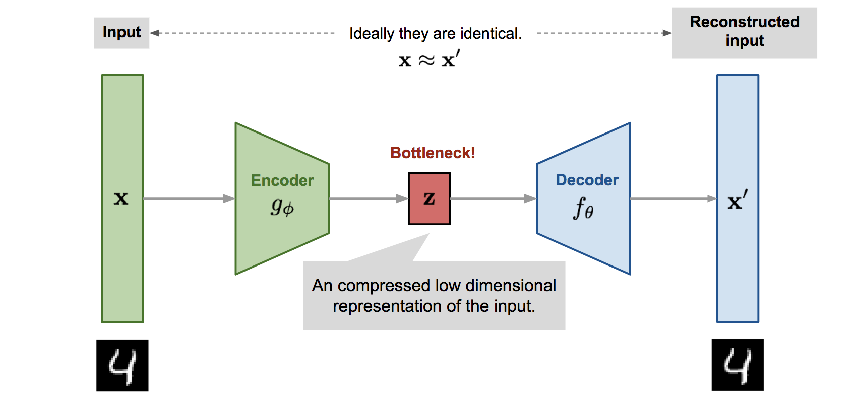
Variational Autoencoders (VAEs) are generative models that combine probability theory with deep learning.
They learn a latent representation $z$ for high-dimensional data $x$ (e.g. images), and allow us to both encode and generate data.

---

1. The Generative Model

We assume the data $x$ is generated from a latent variable $z$:

1. Sample latent code:

   $$z \sim p(z), \quad p(z) = \mathcal{N}(0, I)$$

2. Generate data from decoder:

   $$x \sim p_\theta(x \mid z)$$

Thus, the joint distribution is

$$p_\theta(x,z) = p_\theta(x \mid z) \, p(z).$$

The marginal likelihood of an observation is obtained by integrating over all latent variables:

$$p_\theta(x) = \int p_\theta(x \mid z)\, p(z)\, dz.$$

---

2. The Intractability Problem

Computing $p_\theta(x)$ requires evaluating a high-dimensional integral, which is usually intractable.

We are also interested in the posterior distribution of $z$:

$$p_\theta(z \mid x) = \frac{p_\theta(x \mid z)\, p(z)}{p_\theta(x)}.$$

But since $p_\theta(x)$ is intractable, so is this posterior.

---

3. Variational Approximation

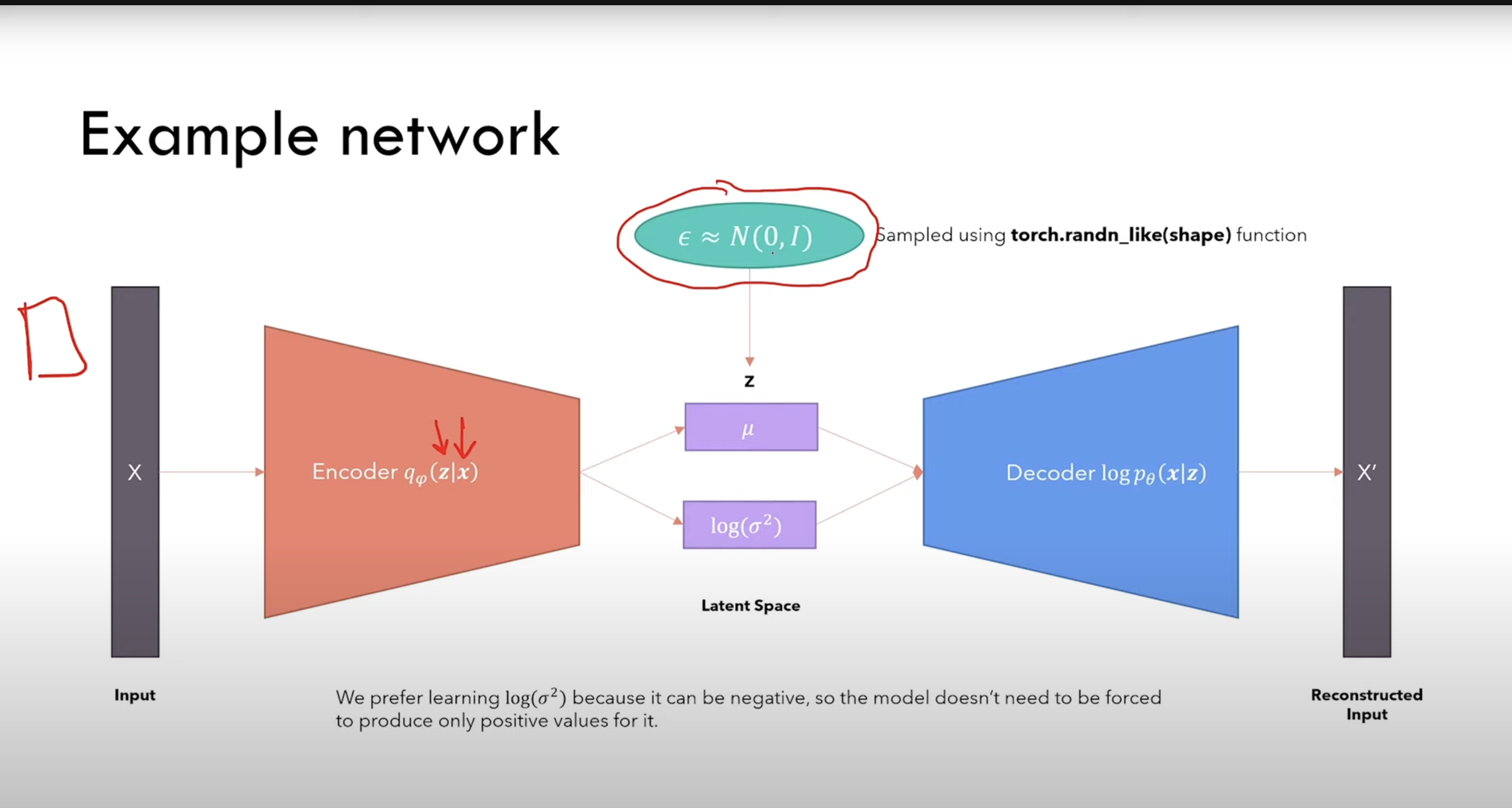
To address this, we introduce an approximate posterior $q_\phi(z \mid x)$, parameterized by an encoder neural network.

The goal is to make $q_\phi(z \mid x)$ close to the true posterior $p_\theta(z \mid x)$.

We measure closeness using the Kullback–Leibler divergence:

$$\mathrm{KL}\!\left(q_\phi(z \mid x) \;\|\; p_\theta(z \mid x)\right) = \mathbb{E}_{q_\phi(z \mid x)} \left[ \log \frac{q_\phi(z \mid x)}{p_\theta(z \mid x)} \right].$$

---

4. Evidence Lower Bound (ELBO)

Starting with the log marginal likelihood:

$$\log p_\theta(x) = \log \int p_\theta(x,z)\,dz.$$

We insert $q_\phi(z \mid x)$ inside the integral:

$$\log p_\theta(x) = \log \int q_\phi(z \mid x)\, \frac{p_\theta(x,z)}{q_\phi(z \mid x)}\, dz.$$

Applying Jensen’s inequality:

$$\log p_\theta(x) \;\geq\; \mathbb{E}_{z \sim q_\phi(z \mid x)} \Big[ \log \tfrac{p_\theta(x,z)}{q_\phi(z \mid x)} \Big].$$

This expectation is the Evidence Lower Bound (ELBO):

$$\mathcal{L}(\theta,\phi; x) = \mathbb{E}_{z \sim q_\phi(z \mid x)} \Big[ \log p_\theta(x \mid z) \Big] - \mathrm{KL}\!\left( q_\phi(z \mid x) \,\|\, p(z) \right).$$

---

5. Alternative Formulation

We can relate the ELBO to the KL divergence with the true posterior:

$$\log p_\theta(x) = \mathcal{L}(\theta,\phi; x) + \mathrm{KL}\!\big(q_\phi(z \mid x) \,\|\, p_\theta(z \mid x)\big).$$

Since KL divergence is always non-negative:

$$\log p_\theta(x) \;\geq\; \mathcal{L}(\theta,\phi; x).$$

Thus, maximizing the ELBO makes $q_\phi(z \mid x)$ approximate the true posterior.

---

6. Concrete Loss Function

• Reconstruction term:

  $$\mathbb{E}_{z \sim q_\phi(z \mid x)} \big[ \log p_\theta(x \mid z) \big]$$

  Encourages the decoder to reconstruct the data correctly.
  In practice, this is a cross-entropy (for Bernoulli pixels) or mean squared error (for Gaussian outputs).

• Regularization term (KL):

  $$\mathrm{KL}\!\big(q_\phi(z \mid x) \,\|\, p(z)\big)$$

  Encourages the approximate posterior to stay close to the Gaussian prior $p(z)=\mathcal{N}(0,I)$.

---

7. The Reparameterization Trick

To make gradients flow through random sampling, we reparameterize:

$$z \sim q_\phi(z \mid x) = \mathcal{N}\big(\mu_\phi(x), \sigma_\phi^2(x) I\big)$$

as

$$z = \mu_\phi(x) + \sigma_\phi(x) \odot \epsilon, \quad \epsilon \sim \mathcal{N}(0, I).$$

This allows backpropagation through $z$.

---

8. Final Training Objective

The training objective for a single data point $x$ is:

$$\mathcal{L}(\theta,\phi; x) = \underbrace{\mathbb{E}_{z \sim q_\phi(z \mid x)} \big[ \log p_\theta(x \mid z) \big]}_{\text{Reconstruction term}} - \underbrace{\mathrm{KL}\!\big(q_\phi(z \mid x) \,\|\, p(z)\big)}_{\text{Regularization term}}.$$

In practice, the expectation is estimated with a single Monte Carlo sample per data point.

---

9. Summary

• $x$ = observed data (e.g., pixels of an image).
• $z$ = latent vector (low-dimensional representation).
• VAE loss = expectation integral (reconstruction) + KL penalty.

$$\boxed{\; \mathcal{L}(\theta,\phi; x) = \int q_\phi(z \mid x)\, \Big[\log p_\theta(x \mid z) - \log \tfrac{q_\phi(z \mid x)}{p(z)}\Big] dz \;}$$

This compact form highlights that VAEs balance reconstruction accuracy with latent space regularity, enabling smooth interpolation and generation of new data.